Step 1
Enter a number in cell A1 and hit the enter key and then click on cell A1Step 2
Click on the Formulas tab in Excel and then click in the “Name Manager” button. The following Window will appear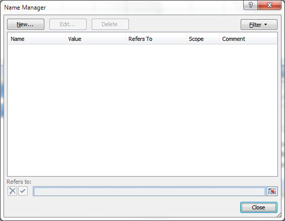
Step 3
In the Name Manager window, click the “New” button and in the Window that appears, type the name “ChartData” in the “Name” textbox and in the “Scope” list box, select “Sheet1” and then enter the following formula in the textbox labeled “Refers to”: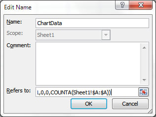
Step 4
Click on the “Insert” tab in the Excel main menu and then in the “Charts” section of the ribbon, click on the type of chart that you want. This will insert a chart in the worksheet.Step 5
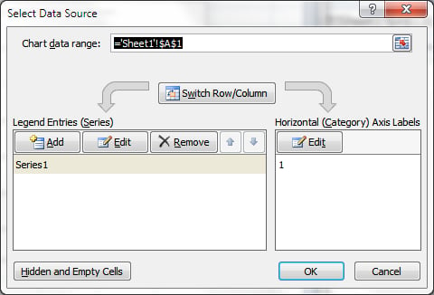
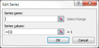
The Design tab should automatically be selected in the Excel main menu. If it is not, select it and then click on the button labeled “Select Data”. This will open a new window: